Sabit ağırlıklı stratejilerin sonu
Kripto piyasasında ilk denemelerim klasik tec stratejileriydi: RSI 30'un altına düşünce al, 70'in üstüne çıkınca sat. Backtest'te güzel sonuç veriyordu. Canlıda ise her ay başka bir indikatör öne çıkıyordu. Piyasa rejimi değişiyor, sabit kurallar geçerliliğini yitiriyordu.
Üçüncü ayda fark ettim ki, hangi indikatörün o ay "doğru" olduğunu bilmiyorum. Sadece geriye dönük bakınca görülebiliyor. Bu, modele dayalı bir yaklaşım gerektiriyor.
Veri ve indikatörler
Pipeline'ın girişi Binance ve Bybit'ten çekilen 5 dakikalık OHLCV mumları. 13 indikatör hesaplıyorum:
- Trend: EMA 9/21/50/200, MACD, ADX
- Momentum: RSI 14, Stochastic RSI, Williams %R
- Volatilite: Bollinger Bands, ATR, Keltner Channels
- Volume: OBV, VWAP
Hedef değişken: bir sonraki 4 saatte en az %0.8 yukarı hareket olup olmayacağı. İkili sınıflandırma problemi olarak ele alıyorum.
İlk denemelerimde inanılmaz yüksek accuracy aldım: %78. Sonra fark ettim ki, EMA 200 gibi uzun vadeli indikatörler henüz gerçekleşmemiş veriye bakıyor. Lookback window'u 200 mumla sınırlayıp, train/test split'i zamansal (rastgele değil) yaptım. Accuracy %62'ye düştü — gerçekçi bir sayı.
XGBoost modeli
Gradient boosting'in XGBoost implementasyonunu seçtim. Sebepleri: hızlı, regularization yerleşik, eksik veriyle iyi başa çıkıyor, feature importance sunuyor.
Temel parametreler: max_depth=6, learning_rate=0.05, n_estimators=400, subsample=0.8. Ama bu sayılar optimal değil. Hiperparametre araması için Bayesian optimization kullanıyorum.
Bayesian optimization
Grid search 4 saat sürüyor ve yerel minimumlerde takılı kalıyor. Bayesian optimization (Optuna kütüphanesi) önceki denemelerden öğrendiği bir prior ile yeni kombinasyonları seçiyor. 50 trial'da, grid search'ün bulduğundan daha iyi parametreler buldu, süre 18 dakikaya indi.
import optuna
def objective(trial):
    params = {
        'max_depth': trial.suggest_int('max_depth', 3, 9),
        'learning_rate': trial.suggest_float('lr', 0.01, 0.3, log=True),
        'n_estimators': trial.suggest_int('n', 100, 800),
        'subsample': trial.suggest_float('sub', 0.6, 1.0),
        'colsample_bytree': trial.suggest_float('col', 0.5, 1.0),
        'reg_alpha': trial.suggest_float('a', 1e-8, 10, log=True),
        'reg_lambda': trial.suggest_float('l', 1e-8, 10, log=True),
    }
    model = xgb.XGBClassifier(**params, early_stopping_rounds=30, eval_metric='auc')
    model.fit(X_train, y_train, eval_set=[(X_val, y_val)], verbose=False)
    return roc_auc_score(y_val, model.predict_proba(X_val)[:, 1])
study = optuna.create_study(direction='maximize')
study.optimize(objective, n_trials=50)
Ensemble
Tek bir model overfit'e meyilli. Bunu çözmek için üç farklı bakış açısıyla üç model eğitiyorum:
- Trend-following: EMA ve MACD ağırlıklı feature subset
- Mean-reversion: RSI ve Bollinger ağırlıklı
- Volume-based: OBV ve VWAP ağırlıklı
Final sinyal: üç modelin tahminlerinin ağırlıklı ortalaması. Ağırlıklar Bayesian optimizasyonla, geriye dönük Sharpe'ı maksimize edecek şekilde belirleniyor. Üç ayda ağırlıklar şöyle stabilize oldu: trend 0.42, mean-rev 0.31, volume 0.27.
Sonuçlar
6 aylık out-of-sample backtest, slippage ve fee'ler dahil:
- Sabit ağırlıklı strateji: Sharpe 1.42, max drawdown %18.4
- XGBoost + Bayesian ensemble: Sharpe 1.95, max drawdown %11.2
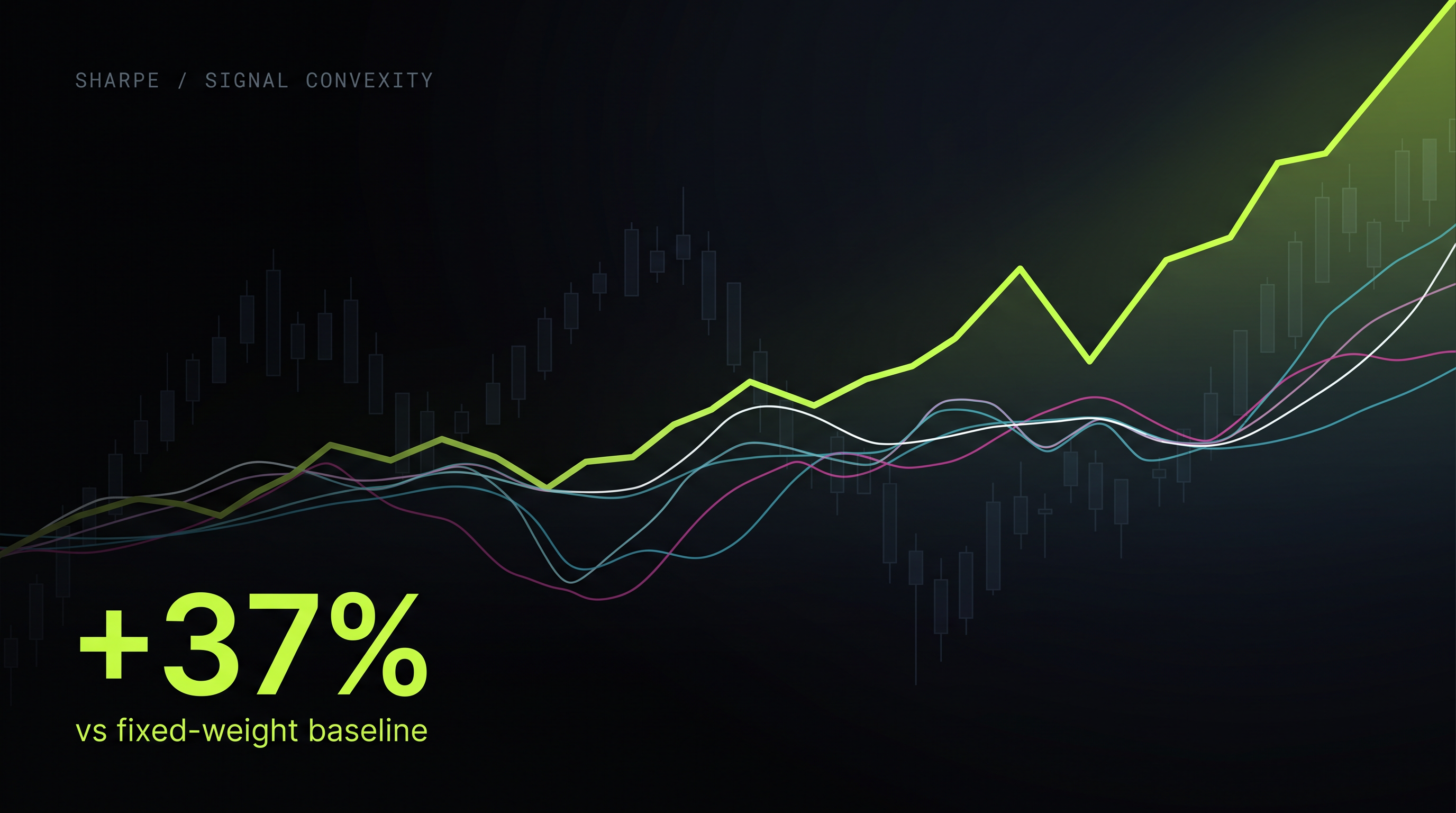
- Kazanç: +%37 Sharpe, -%39 drawdown
Drawdown azalması özellikle önemli. Tek bir model hata yaptığında ağır darbe alıyordum; ensemble'da üç farklı bakış açısı yanlışa yanlış demiyor.
Production'a geçiş
Modeller eğitildikten sonra, canlıda iki kritik unsur var: veri akışı ve hız. FastAPI ile bir servis yazdım: her 5 dakikada bir CCXT üzerinden yeni mumları çekiyor, indikatörleri hesaplıyor, üç modeli çalıştırıyor, ensemble sinyalini üretiyor. Toplam latency 180ms.
Sinyal pozitifse Telegram bot'una mesaj gidiyor. Pozisyon boyutu Kelly Criterion ile belirleniyor ama maksimum %2 equity ile sınırlandırıldı. Drawdown %8'i geçince model durduruluyor, manuel review başlıyor.
Öğrenilenler
En önemli çıkarım: ML modeli tek başına çözüm değil. Veri temizliği, feature engineering, ensemble mimarisi, risk yönetimi — hepsi birlikte çalışıyor. İlk denemede "model accuracy'si yüksek" diye sevindim. Gerçek performans ise ancak tüm pipeline olgunlaşınca ortaya çıktı.
İkinci öğrenim: backtest hileli olabilir. Zamansal split, slippage, fee, latency — hepsini dahil etmeden güvenilir bir metrik alamazsınız. Out-of-sample testi minimum 3 ay tutun.
Üçüncü öğrenim: regime değişimlerine hazırlıklı olun. Model 2024 boğa piyasasında mükemmel çalışırken, 2025 düzeltmesinde Sharpe'ı yarı yarıya düşürdü. Quarterly re-training şart, ama yetmez — piyasa yapısı temelden değiştiğinde (örneğin ETF onayı sonrası) modeli sıfırdan eğitmek gerekiyor.
The end of fixed-weight strategies
My first attempts in crypto were classic TA strategies: buy when RSI drops below 30, sell when it crosses 70. Backtests looked great. In production, a different indicator led the way every month. Market regime shifted, fixed rules became obsolete.
By the third month I realized I had no way of knowing which indicator was "right" that month. You only see it in hindsight. That called for a model-driven approach.
Data and indicators
The pipeline starts with 5-minute OHLCV candles pulled from Binance and Bybit. I compute 13 indicators:
- Trend: EMA 9/21/50/200, MACD, ADX
- Momentum: RSI 14, Stochastic RSI, Williams %R
- Volatility: Bollinger Bands, ATR, Keltner Channels
- Volume: OBV, VWAP
Target: whether the next 4 hours will see at least a 0.8% upward move. Binary classification.
My first runs reported an absurd 78% accuracy. Then I noticed that long-window indicators like EMA 200 were looking at future data. I capped the lookback to 200 candles and switched to a temporal train/test split (not random). Accuracy dropped to 62% — a realistic number.
XGBoost model
I went with the XGBoost implementation of gradient boosting. Fast, regularization built-in, handles missing values gracefully, ships feature importance.
Baseline params: max_depth=6, learning_rate=0.05, n_estimators=400, subsample=0.8. But these aren't optimal. Hyperparameter search needs Bayesian optimization.
Bayesian optimization
Grid search took 4 hours and got stuck in local minima. Bayesian optimization (Optuna) uses a prior learned from past trials to pick new combinations. 50 trials found better params than grid search, in 18 minutes.
import optuna
def objective(trial):
    params = {
        'max_depth': trial.suggest_int('max_depth', 3, 9),
        'learning_rate': trial.suggest_float('lr', 0.01, 0.3, log=True),
        'n_estimators': trial.suggest_int('n', 100, 800),
        'subsample': trial.suggest_float('sub', 0.6, 1.0),
        'colsample_bytree': trial.suggest_float('col', 0.5, 1.0),
        'reg_alpha': trial.suggest_float('a', 1e-8, 10, log=True),
        'reg_lambda': trial.suggest_float('l', 1e-8, 10, log=True),
    }
    model = xgb.XGBClassifier(**params, early_stopping_rounds=30, eval_metric='auc')
    model.fit(X_train, y_train, eval_set=[(X_val, y_val)], verbose=False)
    return roc_auc_score(y_val, model.predict_proba(X_val)[:, 1])
study = optuna.create_study(direction='maximize')
study.optimize(objective, n_trials=50)
Ensemble
A single model tends to overfit. To address that I train three models with three different perspectives:
- Trend-following: feature subset weighted by EMA and MACD
- Mean-reversion: weighted by RSI and Bollinger
- Volume-based: weighted by OBV and VWAP
Final signal: weighted average of the three predictions. Weights are picked by Bayesian optimization to maximize historical Sharpe. After three months, weights stabilized at: trend 0.42, mean-rev 0.31, volume 0.27.
Results
6-month out-of-sample backtest, slippage and fees included:
- Fixed-weight strategy: Sharpe 1.42, max drawdown 18.4%
- XGBoost + Bayesian ensemble: Sharpe 1.95, max drawdown 11.2%
- Gain: +37% Sharpe, -39% drawdown
Drawdown reduction is especially meaningful. With a single model, one bad call could crater the equity curve. The ensemble rarely has all three perspectives agree on the wrong side.
Production deployment
Once models are trained, two critical things in production: data pipeline and latency. I built a FastAPI service that pulls new candles every 5 minutes via CCXT, computes indicators, runs the three models, and produces the ensemble signal. End-to-end latency: 180ms.
If the signal is positive, a Telegram bot gets the message. Position sizing follows Kelly Criterion, capped at 2% of equity. If drawdown exceeds 8%, the model is paused and manual review kicks in.
Lessons learned
The biggest takeaway: an ML model alone isn't the answer. Data cleaning, feature engineering, ensemble architecture, risk management — they all have to work together. I celebrated the first "high accuracy" run. Real performance only emerged once the entire pipeline matured.
Second lesson: backtests can lie. Temporal split, slippage, fees, latency — without all of these you don't have a reliable metric. Hold out-of-sample tests for at least 3 months.
Third lesson: expect regime shifts. The model was great in the 2024 bull run, then halved its Sharpe in the 2025 correction. Quarterly re-training is necessary but not sufficient — when the market structure changes fundamentally (post-ETF approval, for example), the model needs to be retrained from scratch.